Introduction to decision trees

Classification and regression decision trees allow us to investigate some simple mixtures of features. Decision trees are conveniently interpretable, and we can read yes/no decision rules directly off of them. Mixing decision trees, e.g. with the random forests method, has been found to be very effective, so we try this as well.

Like before, we continue to assume that nothing beyond n lookback trials matters. However, unlike before, we no longer assume that there are no interactions between trials; we use CART specifically to enable interactions and to enable non-linear relationships.

Here we use CART and random forests for the binary classification problem of predicting the rat’s next action given several previous actions and rewards. Features are represented as categorical variables, and we validate performance with 5-fold cross-validation. We use scikit-learn’s implementation of decision trees and random forests.

CART procedure

We choose random sessions from a random rat, and then set a lookback number n that encodes how much memory our model has. That is, we incorporate the choices and rewards from the previous n trials when trying to predict the rat’s next choice. Before doing so, we discard forced choice trials – in the future, we need to think carefully about how to incorporate these.

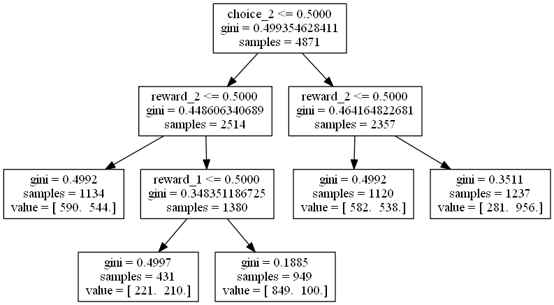
For rat M042, with n=3 (3 trials lookback), and 10 random sessions chosen, we have a decision tree that looks as follows:

Interpreting the tree

Features are labeled as follows:

• choice_n is the choice the rat made n trials ago, where L is labeled as 0 and R is labeled as 1
• reward_n is the reward the rat received n trials ago, i.e. either 0 or 1.

The left arrow from each node represents “true”, and the right arrow represents “false”. samples refers to how many trials are represented by each node, gini is (intuitively) a measure of confusion, and value = [ ... ... ] counts how many Left and how many Right choices are made by the rat next in each leaf node. A low gini score means there is low confusion, i.e. L’s and R’s can be separated relatively cleanly.

For example, we can read off the following rule:

1. If the rat chose L 2 trials ago,
2. and if the rat got a reward 2 trials ago,
3. and if the rat got a reward 1 trial ago,
4. then with low confusion (gini = 0.1863), the rat is more likely to choose L than R next. In fact, the rat chooses L 836 times and R 97 times.

How good is this tree at modeling rat behavior?

We constructed that tree from 1 of 5 cross-validation folds (with the number of L’s and R’s approximately balanced in each fold per the population proportions). On this fold:

• Training accuracy: 0.6565
• Held out accuracy: 0.6519
• Held out ROC AUC: 0.7188

Combining trees: random forests

Let’s combine decision trees by using a random forest binary classifier with 100 estimators, over five cross-validation folds. This is done over the same rat and the same randomly selected sessions as before.

Our results are:

Accuracy: 0.75 (+/- 0.04)
ROC AUC: 0.84 (+/- 0.01)
Average feature importances:
1	reward_1	0.340961
2	choice_1	0.278615
3	choice_2	0.158247
4	reward_2	0.094475
5	choice_3	0.085114
6	reward_3	0.042588

The ROC AUC is much higher than with one decision tree alone.

Varying some parameters

Let’s vary n_lookback, and also use a different rat and different sessions to see what changes. Here are the results:

rat M044
chosen sessions: [ 87  85 120  98  37 130  48 100 138 142]
************************************************************
lookback number: 2
************************************************************

Feature space holds 4222 observations and 4 features
Unique target labels: [0 1]
Accuracy: 0.76 (+/- 0.06)
ROC AUC: 0.83 (+/- 0.02)
Average feature importances:
1	reward_1	0.346253
2	choice_1	0.342026
3	choice_2	0.222051
4	reward_2	0.089670
************************************************************
lookback number: 3
************************************************************

Feature space holds 4212 observations and 6 features
Unique target labels: [0 1]
Accuracy: 0.76 (+/- 0.06)
ROC AUC: 0.83 (+/- 0.02)
Average feature importances:
1	choice_1	0.290650
2	reward_1	0.276047
3	choice_2	0.177881
4	choice_3	0.120302
5	reward_2	0.083337
6	reward_3	0.051782
************************************************************
lookback number: 4
************************************************************

Feature space holds 4202 observations and 8 features
Unique target labels: [0 1]
Accuracy: 0.76 (+/- 0.06)
ROC AUC: 0.81 (+/- 0.03)
Average feature importances:
1	choice_1	0.245800
2	reward_1	0.236073
3	choice_2	0.145665
4	choice_3	0.111321
5	reward_2	0.084063
6	choice_4	0.068400
7	reward_3	0.060731
8	reward_4	0.047948
************************************************************
lookback number: 5
************************************************************

Feature space holds 4192 observations and 10 features
Unique target labels: [0 1]
Accuracy: 0.74 (+/- 0.05)
ROC AUC: 0.80 (+/- 0.02)
Average feature importances:
1	reward_1	0.205319
2	choice_1	0.178853
3	choice_2	0.118502
4	choice_3	0.089454
5	reward_2	0.083608
6	reward_3	0.067823
7	choice_5	0.067702
8	choice_4	0.065747
9	reward_4	0.064158
10	reward_5	0.058832

ROC AUC is highest for n=2 or n=3, but not significantly.

Let’s remove any remaining dependence on rat and sessions.

That is, for many rats and sessions, let’s get average ROC AUCs for each n_lookback. We do this by choosing 10 random rats, and taking the mean ROC AUC from a random forest classifier trained and tested on 5 CV folds across each rat’s 10 random sessions. Then we find the mean and standard deviation of the mean ROC AUC’s.

The results are:

n = 2 : average ROC across folds = 0.8505 (+/- 0.0830)
n = 3 : average ROC across folds = 0.8547 (+/- 0.0861)
n = 4 : average ROC across folds = 0.8472 (+/- 0.0946)
n = 5 : average ROC across folds = 0.8372 (+/- 0.1051)

It seems that $n = 3$ does the best, but not by much.