Week 5
Rat variability
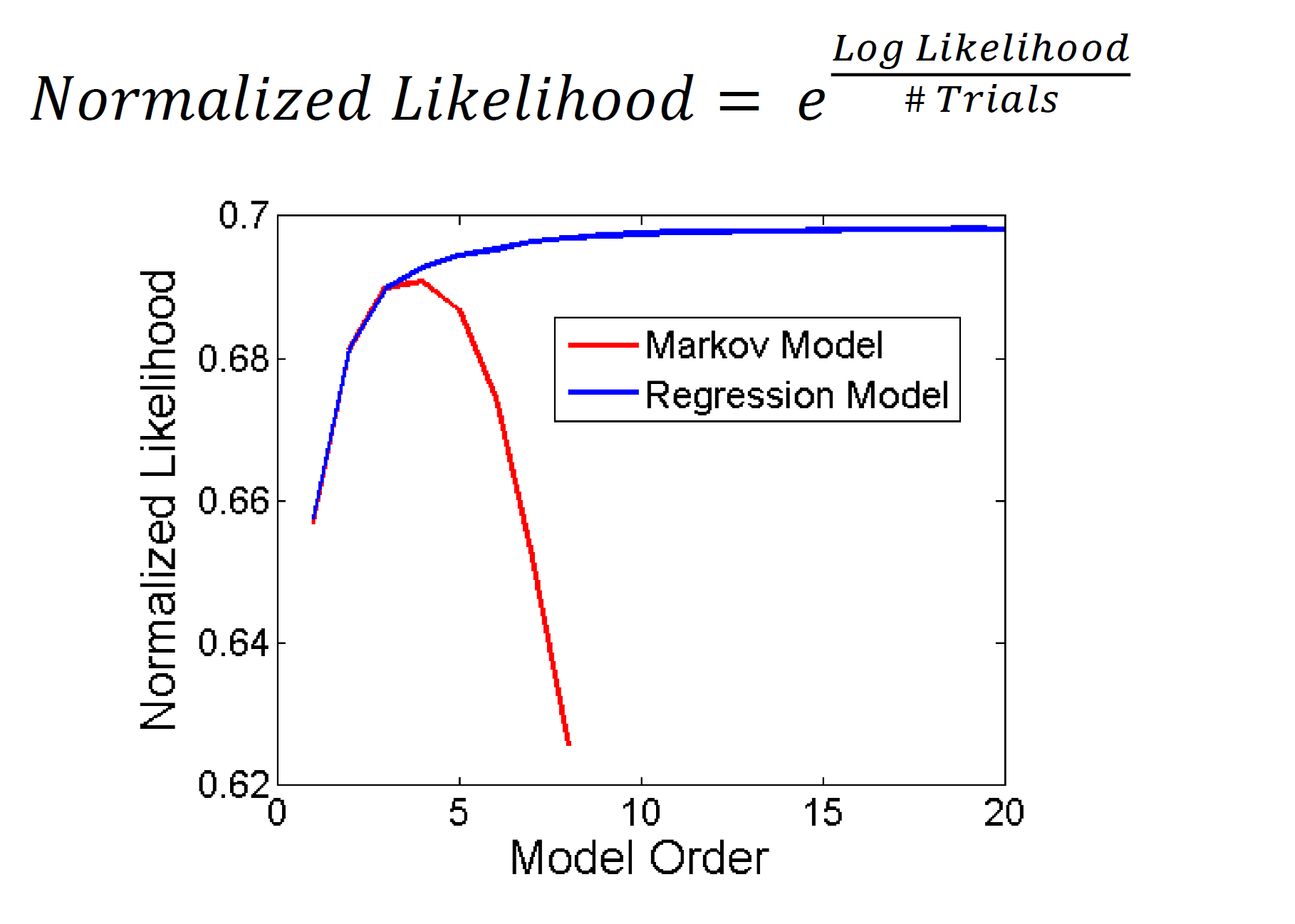
The linear model with reduced number of parameters is as follows. It assumes exponentially decaying memory for the actions that the rat carried out in previous time steps (“habit”) and for the interactions of actions and rewards in previous time steps (“reinforcement learning”). There are 7 total parameters:
- Coefficient $\beta_H$ and decay $\alpha_H$ for habit,
- Coefficient $\beta_{RL}$ and decay $\alpha_{RL}$ for reinforcement learning,
- Coefficient for the action in the previous time step, $\beta_P$ (perseveration),
- Coefficient for the action/reward in the previous time step, $\beta_{WSLS}$ (win-stay-lose-switch),
- Bias term $c$.
In this model, the probability of going left in time step $t$ is given by the logistic function composed with
$$ \sum_{k\ge 2} \beta_{t-k}(1-\alpha_{H})^kA_{t-k} + \sum_{k\ge 2} \beta_{t-k}(1-\alpha_{RL})^kI_{t-k} + \beta_P A_{t-1} + \beta_{WSLS} I_{t-1} + c $$
where $A_i$ denotes the action at time $i$, and $I_i$ denotes the interaction of action and reward at time $i$.
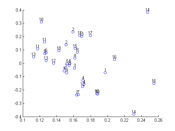
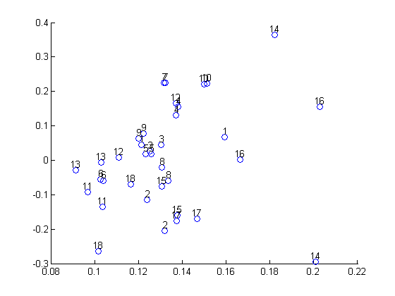
We learn the parameters for each rat’s odd and even trials to get a $36\times 7$ matrix of parameters, 2 for each rat. We center the data and run PCA on this data to see variability between rats. (Technical point: instead of using the $\alpha$’s, we use $\ln(1-\alpha)$, which is the actual decay rate of the exponential.) We run it twice, one without and one with standardizing (dividing by the variance of each parameter after centering).
The amount of variation expained by the top 2 principal components are 87.6%, 8.0% and 89.6%, 6.8%, respectively. We use PCA to reduce the parameters to 2 dimensions. Here are the plots. Note that for most rats, the parameters learned for the even and odd trials are close.
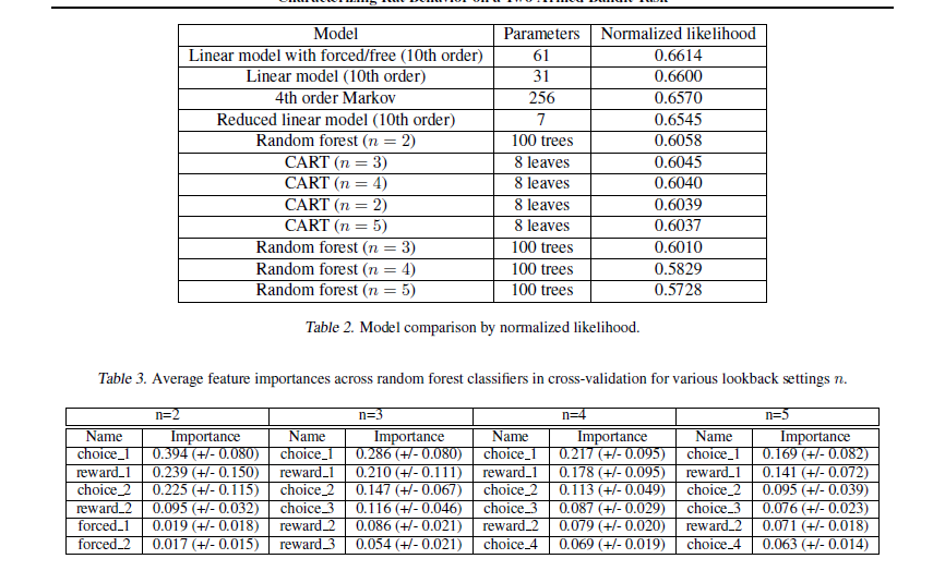
Model comparison, continued: CART vs the world
We are beating the CART / Random Forests baseline: