Methods

We propose 3 methods to analyze the data: Markov models, logistic regression, and CART.

Markov Models

We formally define the Markov model and variants.

• Simple (n+1)th-order Markov model: We observe a time series $A_1,A_2,\ldots$ taking discrete values. The distribution of each $A_t$ depends only on the history of the previous $n$ states $A_{n-t},\ldots, A_{t-1}$. The number of parameters scales as $s^n$, where $s$ is the number of possible states of each $A_t$. In our case, the observations are “L0”, “L1”, “R0”, “R1”, namely the action and the reward, so there are $4^n$ parameters, $\mathbb P(L | \text{past $n$ observations})$. (We don’t attempt to predict the next reward, just the next action.) The large number of parameters makes this model prone to overfitting.
• Online Markov model (Stream coding): Rather than predict the Markov model given all the data, at each step predict the next state given the previous $n$ states, using only the data so far.
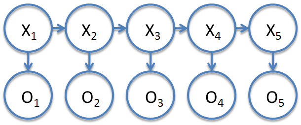
• Hidden Markov Model: We see a series of observations $O_1,O_2,\ldots$; however, we do not take these observations as states of the Markov chain. We assume that each time step is associated to a state $X_t$ of the Markov chain. The parameters are ** A transition matrix of probabilities $A$ that gives the probabilities $\mathbb P(X_{t+1}|X_t)$. ** A matrix $B$ of probabilities of observations $\mathbb P(O_t,X_t)$. (The number of states must be set or inferred.)

Validation: For the Markov model and hidden Markov model, estimate the probability using a subset of the data, and then test its performance on the rest. The loss function is the average “surprise”, where the surprise at time $t$ is $-\lg p$ if the algorithm predicted the result with probability $p$ (This is basically a log likelihood). For the online Markov model, the fact that it only sees the previous observations means no further validation is necessary.

Limitations: The simple Markov model assumes that only the previous $n$ trials influence the decision. Furthermore, the state space is discrete in all cases, so cannot model the rat having a “continuous” variable in memory.

Algorithm: For the simple Markov model, simply estimate the probabilities empirically (possibly with a normalization factor). For HMM’s it is intractable to find the parameters with max likelihood. In practice, the EM (Baum-Welch) algorithm is used; also there are spectral methods that predict the next observation without inferring the underlying parameters.

Online Markov Model (Stream coding)

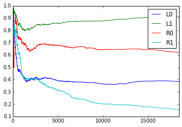
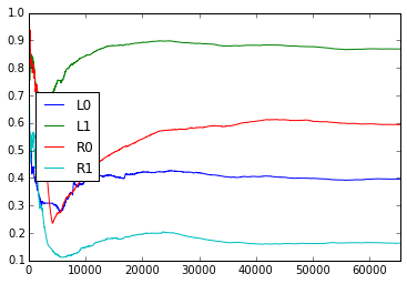
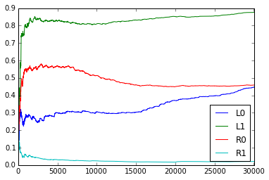
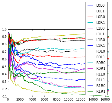
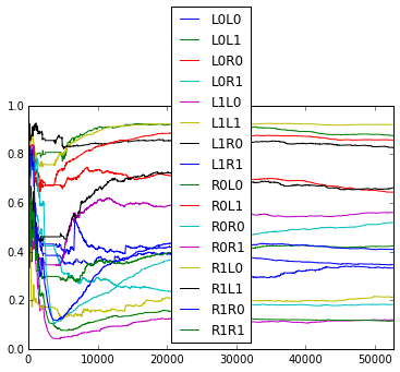
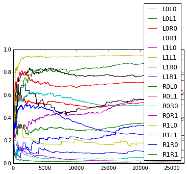
How do the empirical transition probabilities change over time? Here are graphs showing how the empirical probabilities change over time (for example, the plot for ‘L0L0’ is $\frac{L0L0L + 1}{L0L0L + L0L0R + 2}$ where the count is only over the past trials). The graphs fluctuate somewhat, but it seems unclear whether they are random or there is more pattern in the fluctuations.

The average surprise for 2 rats for the 1st through 5th order online model are as follows.

Order	Rat 1	Rat 2
1	0.9980053667619428	0.9994585193680784
2	0.7150382790620436	0.7616167440739513
3	0.6791163319477521	0.7075967675012327
4	0.666331209801937	0.6868778097403748
5	0.6759193086271804	0.6856632883745152

Here a score of 0 means perfect prediction, and a score of 1 means it does no better than random. It seems that a 4th or 5th order model (i.e., looking at past 3 or 4 trials) does best.

Logistic regression/Generalized linear model

The generalized linear model is as follows. Given values of features $X_i$ at time $t$, choose ‘L’ as the next action with probability $\frac{\exp(a_i X_i)}{\sum_j \exp(a_j X_j)}$. Here the $X_i$ are summaries of previous trials that the rat could use to make its decision, such as

• whether the rat got a reward $k$ trials back,
• whether the rat went left or right $k$ trials back,
• the interaction between the reward and the action (i.e., the XOR of the above two features) $k$ trials back

for $k$ from 1 to 10, say. This has the advantage that the number of parameters scales linearly with the lookback time, rather than exponentially, so is not as prone to overfitting. We can also have more sophisticated models for the $X_i$, such as it being a exponentially weighted sum of previous rewards/actions.

Note that both the naive Markov Model and this model assume that only the past few trials matter in the rat’s next decision.

Max likelihood

The typical way to optimize the constants $a_i$ is by using gradient descent on the log likelihood $-\log( \frac{\exp(a_iX_i)}{\sum \exp(a_jX_j)})$, either stochastically or on the sum over all trials. This is a convex function, so we have good convergence guarantees.

Bayesian perspective

Alternatively, we can put priors on the $a_i$, and then find the posterior distribution after observing the rat’s trials. This perspective may be more helpful when we have a lot of features and assume that only a few of them actually matter.